Genetic optimization: searching a million combinations

Every systematic strategy has parameters: moving-average lengths, entry thresholds, stop-loss multiples, timeframes. And for each parameter there is a natural question: what if it were somewhere else? The wrong answer is to try by hand and stop when the numbers look pretty. The right answer is to explore the whole space of settings systematically — and our platform has two tools for exactly that: an exact grid and genetic optimization.

The exact grid: every value against every other

Give the parameters ranges (from–to, with a step) and a lattice of combinations appears. Grid search sweeps it whole: every variable parameter against all the others, every value against every value. No blind spots, no chance — a complete map. Thanks to a fast event-driven engine, thousands of full backtests are routine, so for smaller spaces the grid is the first choice.

But combinatorics is merciless: four parameters with ten values each = 10⁴ = 10,000 tests. Six parameters with twelve values = almost 3 million. Somewhere along that road brute force stops being practical — and that is precisely where genetic optimization lives up to its name.

Genetics: evolution instead of brute force

Genetic optimization is an evolutionary method of searching a strategy's parameter space: instead of trying every combination, it breeds a population of candidates by a chosen metric — generation after generation, toward the regions where the strategy works.

A genetic algorithm does not try everything — it breeds. It starts with a population of random candidates scattered across the whole space. Each candidate (a “chromosome”) is one concrete strategy setting — and each is scored with a full backtest: real execution simulation, fees and slippage included, no shortcuts. The result yields a fitness — a score by the chosen metric. Then evolution kicks in: the successful reproduce, the unsuccessful vanish, offspring combine their parents' traits and occasionally mutate. Generation by generation, the population converges toward the regions where the strategy works.

The landscape is not free, though — and it matters what it cost. We also track how many tests and combinations it took before the optimization reached good results. When a huge number of attempts leaves only a small cluster or a handful of “optimal” tests, that is not an optimal solution — it is a warning. And it is just as important to judge the results through several metrics at once: we are looking for a robust landscape, not a spiky mountain range with deep valleys.

One generation up close. The roulette gives odds proportional to fitness — even a weaker candidate occasionally gets a say (protecting diversity). The cut point splits the parents, children combine their halves, mutation rewrites one value — and the elite (★) travels down the right-hand rail into the new generation unchanged.

An evolution glossary

Chromosome — one concrete setting: a combination of values of all variable parameters.
Population — the set of candidates of one generation. Each is tested with its own backtest.
Generation — one round of the cycle: test → score → select → cross → mutate.
Fitness — the number evolution selects by. We convert the chosen metric to a 0–1000 score so candidates compare cleanly.
Selection — picking parents by roulette: the higher the fitness, the better the odds of offspring. Even weaker candidates get a chance — that protects diversity.
Crossover — two parents exchange parts of their settings, producing offspring that combine traits of both.
Mutation — a random value change in an offspring. A small dose of chaos that keeps the population from getting stuck in one valley.
Elitism — the best individuals pass to the next generation unchanged, immune to crossover and mutation. What evolution has found once, it never loses.

What gets optimized: fitness metrics

“Best” always means “best by something”. You choose the fitness metric by what you want from the strategy:

Net profit (% PnL) — the most direct, and the most naive, target,
PROM — Pardo's pessimistic return on margin: a result deliberately discounted for statistical luck,
Sharpe and Sortino — return weighted by volatility (Sortino punishes only the downside),
Calmar — return measured against maximum drawdown,
composite metrics — combinations of captured market movement, consistency and drawdown.

We annualize the ratio metrics over 365 days — the markets we trade do not sleep on weekends. What each metric really says, and when it lies, is a separate article: Metrics: how to tell a good strategy from a lucky one.

And how should the fitness be chosen? Our analyses are unambiguous: you will not get the most robust solution by breeding purely for a profit metric — you will breed gamblers. But optimizing purely for drawdown does not work either: such an algorithm starts rejecting any trading that could even contribute to an equity dip — and breeds a strategy that prefers not to trade at all. The right answer is a combination: risk-weighted, penalized metrics — typically PROM or composite scores.

One instrument, or a whole universe

You can optimize on a single market — or on a whole universe of instruments: a basket of markets that meet the strategy's conditions. A candidate then is not graded on how well it fits bitcoin, but on how it holds up across the basket — a much stricter exam (we covered the levels of composition in strategy portfolios). Universes deserve their own article — how they are defined, how strategies built on them work, and how to defend against survivorship bias. It is in the works.

The result: a landscape, not a winner

The most valuable thing about a finished optimization is not row number one. It is the shape of the whole result landscape: where clusters of working settings form, where the plateaus are, where the strategy earns across many neighbouring variants — and where lone peaks stick out that work in a single point only. A plateau means robustness; a peak almost certainly means overfitting. That is why we read results through profit-versus-drawdown scatter plots, clusters and parameter maps — we look for where the strategy works, not which number won.

Clusters and plateaus

Every dot is one candidate. Contiguous clusters (plateaus) mean robustness — many neighbouring settings work. The lone peak at the top right is almost certainly overfitting.

How to read a PCP

The principle of parallel coordinates: every vertical axis is one quantity, every line one test — crossing each axis at its value. Bundles of similar lines = clusters; the right-hand shape of a line tells you at what cost the profit was made.

The live ETH/USDC grid

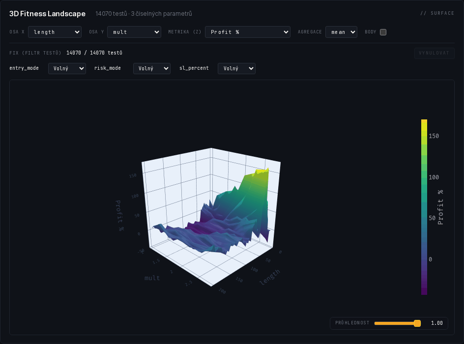
And here is that landscape, live. Not an illustration — a real, completed exact grid of one of our trend-following templates on the ETH/USDC pair (Binance): 14,070 parameter combinations, not a single run failed. The charts show the length band up to 60, where the main action of the landscape happens (multiplier unrestricted); the rendering is the same as in our platform. Try it: in the first chart, drag along a vertical axis to filter candidates (say, low drawdowns only); the second one rotates with your mouse.

Every line = one candidate (a full backtest). Parameters on the left, results on the right: PnL %, max drawdown, time in market, fitness. Drag along an axis to filter. Colour = PnL %: red loss · orange zero · green profit. The default view shows profitable candidates only — stretch the selection on the PnL % axis, or click outside it to clear.

Metric (Z) Aggregate Points

The 3D landscape exactly as in the platform: the surface is the chosen metric for every length × multiplier combination (max/mean/min aggregation across the remaining parameters, gaps filled by neighbour diffusion). Rotate with the mouse; “Points” shows the real cells with test counts.

What the complete grid showed: in the length band up to 60, 1,835 of 4,200 candidates (44 %) finished profitable. The most robust plateau sits at lengths ~23–35 with multipliers 2.2–2.8 — cell-average PnL of 130–170 % — and the single best run (+184.6 %) lies right on its ridge: the winner is not a lone tower but the top of a contiguous plateau. Long lengths, by contrast, form a vast dead plain around zero. That is exactly the shape we look for — and exactly a conclusion for walk-forward, not a ticket to live trading.

3D Fitness Landscape directly from the BXF platform: Viridis surface of Profit % over length × mult axes with axis, metric, aggregation and FIX filter controls — And a view straight into the platform — **the complete grid** (14,070 tests, averaged across the remaining parameters, full length range up to 200). **A good, robust landscape** is a long ridge or a plateau: here lengths ~10–30, where profit holds its height across neighbouring settings. **The warning signs** are lone sharp peaks above deep valleys — performance standing on a single combination. The FIX filters additionally condition the landscape on the remaining parameters.

Genetics as a building block of orchestration

And now the most important part: genetic optimization is one of the first phases of testing, not the last. We never take the best — that is, the most optimal and therefore most likely overfitted — test and say “thanks, bye, going live”. The most promising regions of the landscape continue into walk-forward — and here the power of the orchestration shows: every in-sample window of the walk-forward is itself a genetic optimization. On each slice of history its own evolution runs, its winning settings are verified blind on the following out-of-sample slice, the window rolls forward and everything repeats. Add Monte Carlo on top of the results — and one strategy has thousands of backtests behind it, managed by the platform as a single whole: queues, parallel runs, aggregated results. That is what testing you can trust looks like.

Platform #genetics #optimization

Reading Robert Pardo: The Evaluation and Optimization of Trading Strategies (Wiley) — including the PROM metric. Related articles: Metrics · Walk-forward · Overfitting · Monte Carlo.

Want to see the result landscape of your strategy? Contact us →